贝塞尔曲线:数学推导与Python实现
声明:本学习笔记使用基于GNU TeXmacs的专业编辑工具和python环境实现,内容来自于网络整理学习,内嵌代码由AI辅助并手动调试通过,尽管为了上传做了手动处理,奈何兼容性欠佳,无法实现原开发环境浏览效果。
1. 伯恩斯坦基函数
1.1 数学定义
伯恩斯坦基函数是贝塞尔曲线的数学基础。对于非负整数 n 和整数 i(0≤i≤n),第 i 个 n 次伯恩斯坦基函数定义为:
Bi,n(t)=ti(1-t)n-i
其中:
-
阶数(degree) n:曲线次数
-
索引(index) i:基函数编号
-
参数(parameter) t:取值范围 [0,1]
-
二项式系数(binomial coefficient) =n!i!(n-i)!
1.2 公式推导
伯恩斯坦基函数由二项式定理推导而来。二项式定理指出:
(a+b)n=∑i=0naibn-i
令 a=t,b=1-t,则:
1=(t+(1-t))n=∑i=0nti(1-t)n-i
这正是伯恩斯坦基函数的和,表明它们是单位分割的基函数。
伯恩斯坦基函数还具有递推关系:
Bi,n(t)=(1-t)Bi,n-1(t)+tBi-1,n-1(t)
1.3 代码实现
>>> |
import numpy as np import matplotlib.pyplot as plt from scipy.special import comb import sympy as sp # 设置全局字体为支持中文的字体 plt.rcParams['font.sans-serif'] = ['Microsoft YaHei'] # 使用黑体 plt.rcParams['axes.unicode_minus'] = False # 解决负号显示问题 |
>>> |
def bernstein_basis_numeric(n, i, t):
    """
    计算伯恩斯坦基函数的数值
    """
    return comb(n, i) * (t**i) * ((1-t)**(n-i))
|
>>> |
def plot_bernstein_polynomials():
    """
    绘制伯恩斯坦多项式
    """
    n = 4  # 阶数
    t = np.linspace(0, 1, 200)

    # 创建图形
    fig, axes = plt.subplots(2, 3, figsize=(12, 8))
    axes = axes.flatten()

    for i in range(n+1):
        # 计算基函数值
        B = bernstein_basis_numeric(n, i, t)

        # 绘制图形
        ax = axes[i]
        ax.plot(t, B, 'b-', linewidth=2.5, label=f'$B_{{{i},{n}}}(t)$')
        ax.fill_between(t, 0, B, alpha=0.2)

        # 设置图形属性
        ax.set_xlabel('t', fontsize=12)
        ax.set_ylabel('值', fontsize=12)
        ax.set_title(f'$B_{{{i},{n}}}(t)$', fontsize=14)
        ax.grid(True, alpha=0.3)
        ax.set_xlim(0, 1)
        ax.set_ylim(0, 1)

    # 验证单位分割性质
    ax_sum = axes[5]
    sum_B = np.sum([bernstein_basis_numeric(n, i, t) for i in range(n+1)], axis=0)
    ax_sum.plot(t, sum_B, 'r-', linewidth=2.5, label='和')
    ax_sum.axhline(y=1, color='k', linestyle='--', alpha=0.5)
    ax_sum.set_xlabel('t', fontsize=12)
    ax_sum.set_ylabel(r'$\sum B_{i,n}(t)$', fontsize=12)
    ax_sum.set_title('单位分割性质', fontsize=14)
    ax_sum.grid(True, alpha=0.3)
    ax_sum.set_xlim(0, 1)
    ax_sum.set_ylim(0.99, 1.01)

    fig.suptitle(f'{n}次伯恩斯坦基函数', fontsize=16, fontweight='bold')
    fig.tight_layout()
    return fig
|
1.4 结果输出
>>> |
# 执行绘图 fig_bernstein = plot_bernstein_polynomials() fig_bernstein |
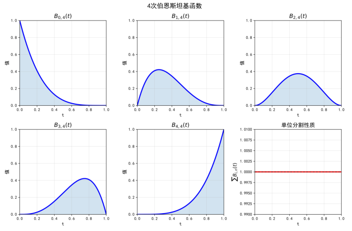
图1:4次伯恩斯坦基函数。每个基函数在 [0,1] 区间上非负,且所有基函数的和为1,满足单位分割性质。
2. 标准(多项式)贝塞尔曲线
2.1 数学定义
给定 n+1 个控制点 P0,P1,…,Pn∈ℝd(通常 d=2 或 3),n 次标准贝塞尔曲线定义为:
C(t)=∑i=0nBi,n(t)Pi=∑i=0nti(1-t)n-iPi
其中 t∈[0,1]。
2.2 公式推导
2.2.1 从线性插值推导(德卡斯特里奥算法)
德卡斯特里奥算法提供了一种递归计算贝塞尔曲线点的方法:
-
对于 t∈[0,1],在线段 PiPi+1 上取点 Pi1(t)=(1-t)Pi+tPi+1
-
在线段 Pi1Pi+11 上取点 Pi2(t)=(1-t)Pi1+tPi+11
-
重复此过程 n 次,得到 P0n(t),即曲线上的点 C(t)
2.2.2 从二项式定理推导
利用二项式定理 (a+b)n=∑i=0naibn-i,令 a=t,b=1-t,得到:
1=(t+(1-t))n=∑i=0nti(1-t)n-i
每个控制点乘以相应的伯恩斯坦基函数,得到曲线方程。
2.3 数学性质
2.3.1 端点性质
-
端点插值:
C(0)=P0,C(1)=Pn
曲线始终通过第一个和最后一个控制点。
-
端点切线:
C'(0)=n(P1-P0),C'(1)=n(Pn-Pn-1)
曲线在端点的切线方向由相邻控制点决定。
-
端点曲率:
C''(0)=n(n-1)(P2-2P1+P0)
曲线在端点的曲率由前三个控制点决定。
2.3.2 凸包性质
凸包是包含所有点的最小凸多边形。对于任意 t∈[0,1],C(t) 位于控制点的凸包内。
证明:由于伯恩斯坦基函数非负且和为1,C(t) 是控制点的凸组合。
2.3.3 仿射不变性
对于任何仿射变换 T:
T(∑i=0nBi,n(t)Pi)=∑i=0nBi,n(t)T(Pi)
2.3.4 变差缩减性
任何直线与贝塞尔曲线的交点数不超过该直线与控制多边形的交点数。
2.4 代码实现
>>> |
def compute_bezier_curve(control_points, t_values=None):
    """
    计算标准贝塞尔曲线

    参数:
    control_points: 控制点数组,形状为 (n+1, 2) 或 (n+1, 3)
    t_values: 参数值数组,默认为 [0, 1] 区间上的100个点

    返回:
    曲线点数组
    """
    control_points = np.array(control_points)
    n = len(control_points) - 1

    if t_values is None:
        t_values = np.linspace(0, 1, 100)

    curve_points = np.zeros((len(t_values), control_points.shape[1]))

    for i, t in enumerate(t_values):
        for j in range(n+1):
            basis = bernstein_basis_numeric(n, j, t)
            curve_points[i] += basis * control_points[j]

    return curve_points
|
>>> |
def de_casteljau_algorithm(control_points, t):
    """
    德卡斯特里奥算法

    参数:
    control_points: 控制点数组
    t: 参数值

    返回:
    曲线在参数t处的点
    """
    points = control_points.copy()
    n = len(points) - 1

    for r in range(1, n+1):
        for i in range(n-r+1):
            points[i] = (1-t) * points[i] + t * points[i+1]

    return points[0]
|
>>> |
def plot_bezier_curve_example():
    """
    绘制标准贝塞尔曲线示例
    """
    # 定义控制点
    control_points_list = [
        np.array([[0, 0], [1, 2], [3, 0]]),  # 二次贝塞尔曲线
        np.array([[0, 0], [1, 3], [2, -1], [4, 2]]),  # 三次贝塞尔曲线
        np.array([[0, 0], [1, 2], [2, -1], [3, 3], [5, 0]])  # 四次贝塞尔曲线
    ]

    titles = ['二次贝塞尔曲线 (n=2)', '三次贝塞尔曲线 (n=3)', '四次贝塞尔曲线 (n=4)']

    # 创建图形
    fig, axes = plt.subplots(1, 3, figsize=(15, 5))

    for idx, (control_points, title) in enumerate(zip(control_points_list, titles)):
        ax = axes[idx]

        # 计算曲线点
        curve_points = compute_bezier_curve(control_points)

        # 绘制控制多边形
        ax.plot(control_points[:, 0], control_points[:, 1],
                'ro-', linewidth=1.5, markersize=8, label='控制多边形')

        # 绘制控制点标签
        for i, point in enumerate(control_points):
            ax.text(point[0]+0.05, point[1]+0.05, f'$P_{i}$',
                   fontsize=12, fontweight='bold')

        # 绘制贝塞尔曲线
        ax.plot(curve_points[:, 0], curve_points[:, 1],
                'b-', linewidth=2.5, label='贝塞尔曲线')

        # 使用德卡斯特里奥算法计算曲线上的点
        t_values = [0.25, 0.5, 0.75]
        for t in t_values:
            point = de_casteljau_algorithm(control_points, t)
            ax.scatter(point[0], point[1], s=80, c='green',
                      edgecolors='black', linewidth=2, zorder=5)
            ax.text(point[0]+0.05, point[1]+0.05, f't={t}',
                   fontsize=10, fontweight='bold')

        ax.set_title(title, fontsize=14, fontweight='bold')
        ax.set_xlabel('x', fontsize=12)
        ax.set_ylabel('y', fontsize=12)
        ax.grid(True, alpha=0.3)
        ax.legend(loc='best')
        ax.axis('equal')

    fig.suptitle('标准贝塞尔曲线示例', fontsize=16, fontweight='bold')
    fig.tight_layout()
    return fig
|
2.5 结果输出
>>> |
# 执行绘图 fig_bezier = plot_bezier_curve_example() fig_bezier |
537 msec
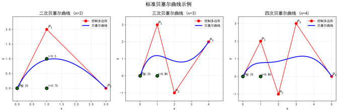
图2:不同阶数的标准贝塞尔曲线。从左到右:二次、三次、四次贝塞尔曲线。曲线始终位于控制多边形形成的凸包内。
3. 有理贝塞尔曲线
3.1 数学定义
有理贝塞尔曲线是标准贝塞尔曲线的推广,每个控制点 Pi 关联一个权重 wi>0。n 次有理贝塞尔曲线定义为:
R(t)=∑i=0nwiBi,n(t)Pi∑i=0nwiBi,n(t)=∑i=0nRi,n(t)Pi
其中有理伯恩斯坦基函数:
Ri,n(t)=wiBi,n(t)∑j=0nwjBj,n(t)
3.2 公式推导
有理贝塞尔曲线可以通过齐次坐标推导。在齐次坐标中,每个控制点表示为 P∼i=(wixi,wiyi,wizi,wi)。曲线在齐次坐标下为:
R∼(t)=∑i=0nBi,n(t)P∼i
通过透视除法得到欧几里得坐标:
R(t)=(x∼(t)w∼(t),y∼(t)w∼(t),z∼(t)w∼(t))
当所有权重相等时,有理贝塞尔曲线退化为标准贝塞尔曲线。
3.3 数学性质
-
投影不变性:在投影变换下保持不变
-
端点插值:R(0)=P0,R(1)=Pn(假设 w0,wn>0)
-
凸包性:曲线位于控制点的凸包内
-
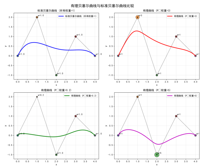
权重影响:wi 增大时,曲线被拉向控制点 Pi
-
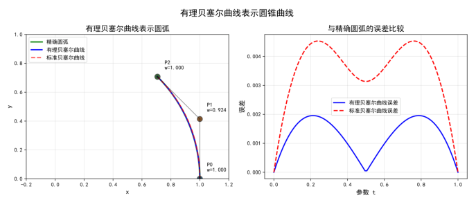
精确表示圆锥曲线:可以精确表示圆、椭圆、抛物线、双曲线
3.4 代码实现
>>> |
def compute_rational_bezier_curve(control_points, weights, t_values=None):
    """
    计算有理贝塞尔曲线

    参数:
    control_points: 控制点数组
    weights: 权重数组
    t_values: 参数值数组

    返回:
    曲线点数组
    """
    control_points = np.array(control_points)
    weights = np.array(weights)
    n = len(control_points) - 1

    if t_values is None:
        t_values = np.linspace(0, 1, 100)

    curve_points = np.zeros((len(t_values), control_points.shape[1]))

    for i, t in enumerate(t_values):
        numerator = np.zeros(control_points.shape[1])
        denominator = 0.0

        for j in range(n+1):
            basis = bernstein_basis_numeric(n, j, t)
            weighted_basis = weights[j] * basis
            numerator += weighted_basis * control_points[j]
            denominator += weighted_basis

        if denominator != 0:
            curve_points[i] = numerator / denominator

    return curve_points
|
>>> |
def plot_rational_bezier_comparison():
    """
    比较有理贝塞尔曲线和标准贝塞尔曲线
    """
    # 定义控制点
    control_points = np.array([
        [0, 0],
        [1, 2],
        [2, -1],
        [3, 1],
        [4, 0]
    ])

    # 定义权重配置
    weight_configs = [
        {'weights': np.ones(5), 'label': '标准贝塞尔曲线 (所有权重=1)', 'color': 'b'},
        {'weights': np.array([1, 3, 1, 1, 1]), 'label': '有理曲线 (P₁权重=3)', 'color': 'r'},
        {'weights': np.array([1, 0.2, 1, 1, 1]), 'label': '有理曲线 (P₁权重=0.2)', 'color': 'g'},
        {'weights': np.array([1, 1, 5, 1, 1]), 'label': '有理曲线 (P₂权重=5)', 'color': 'm'}
    ]

    # 创建图形
    fig, axes = plt.subplots(2, 2, figsize=(12, 10))
    axes = axes.flatten()

    for idx, config in enumerate(weight_configs):
        ax = axes[idx]
        weights = config['weights']

        # 计算曲线
        if np.all(weights == 1):
            curve = compute_bezier_curve(control_points)
        else:
            curve = compute_rational_bezier_curve(control_points, weights)

        # 绘制控制多边形
        ax.plot(control_points[:, 0], control_points[:, 1],
                'ko-', linewidth=1, markersize=6, alpha=0.5)

        # 绘制控制点(大小表示权重)
        for i, (point, weight) in enumerate(zip(control_points, weights)):
            ax.scatter(point[0], point[1], s=weight*80,
                      alpha=0.7, edgecolors='black', linewidth=1)
            ax.text(point[0]+0.05, point[1]+0.05, f'w={weight}',
                   fontsize=10, fontweight='bold')

        # 绘制曲线
        ax.plot(curve[:, 0], curve[:, 1],
                config['color'] + '-', linewidth=2.5, label=config['label'])

        ax.set_title(config['label'], fontsize=12, fontweight='bold')
        ax.set_xlabel('x', fontsize=12)
        ax.set_ylabel('y', fontsize=12)
        ax.grid(True, alpha=0.3)
        ax.legend(loc='best')
        ax.axis('equal')

    fig.suptitle('有理贝塞尔曲线与标准贝塞尔曲线比较', fontsize=16, fontweight='bold')
    fig.tight_layout()
    return fig
|
>>> |
def plot_rational_bezier_circle():
    """
    使用有理贝塞尔曲线绘制圆弧
    """
    # 使用有理贝塞尔曲线表示90度圆弧
    theta = np.pi / 4  # 45度
    r = 1.0  # 半径
    # 控制点坐标
    P0 = np.array([r, 0])
    P1 = np.array([r, r * np.tan(theta/2)])
    P2 = np.array([r * np.cos(theta), r * np.sin(theta)])
    # 权重计算(用于精确表示圆弧)
    w0 = 1.0
    w1 = np.cos(theta/2)
    w2 = 1.0
    control_points = np.array([P0, P1, P2])
    weights = np.array([w0, w1, w2])
    # 计算有理贝塞尔曲线
    t_values = np.linspace(0, 1, 100)
    curve = compute_rational_bezier_curve(control_points, weights, t_values)
    # 计算标准贝塞尔曲线(用于比较)
    std_curve = compute_bezier_curve(control_points, t_values)
    # 精确圆弧
    arc_theta = np.linspace(0, theta, 100)
    exact_arc = np.column_stack([r * np.cos(arc_theta), r * np.sin(arc_theta)])
    # 创建图形
    fig, (ax1, ax2) = plt.subplots(1, 2, figsize=(12, 5))
    # 左图:曲线比较
    ax1.plot(exact_arc[:, 0], exact_arc[:, 1], 'g-',
             linewidth=3, alpha=0.7, label='精确圆弧')
    ax1.plot(curve[:, 0], curve[:, 1], 'b-',
             linewidth=2, label='有理贝塞尔曲线')
    ax1.plot(std_curve[:, 0], std_curve[:, 1], 'r--',
             linewidth=2, alpha=0.7, label='标准贝塞尔曲线')
    # 绘制控制多边形
    ax1.plot(control_points[:, 0], control_points[:, 1],
             'ko-', linewidth=1, markersize=8, alpha=0.5)
    # 标记控制点
    for i, (point, weight) in enumerate(zip(control_points, weights)):
        ax1.scatter(point[0], point[1], s=weight*100,
                   alpha=0.7, edgecolors='black', linewidth=1)
        ax1.text(point[0]+0.05, point[1]+0.05, f'P{i}\nw={weight:.3f}',
                fontsize=10, fontweight='bold')
    ax1.set_xlabel('x', fontsize=12)
    ax1.set_ylabel('y', fontsize=12)
    ax1.set_title('有理贝塞尔曲线表示圆弧', fontsize=14, fontweight='bold')
    ax1.grid(True, alpha=0.3)
    ax1.legend(loc='best')
    ax1.axis('equal')
    ax1.set_xlim(-0.2, 1.2)
    ax1.set_ylim(-0.2, 1.2)
    # 右图:误差分析
    # 计算误差
    error_rational = np.linalg.norm(curve - exact_arc, axis=1)
    error_standard = np.linalg.norm(std_curve - exact_arc, axis=1)
    ax2.plot(t_values, error_rational, 'b-', linewidth=2,
             label='有理贝塞尔曲线误差')
    ax2.plot(t_values, error_standard, 'r--', linewidth=2,
             label='标准贝塞尔曲线误差')
    ax2.set_xlabel('参数 t', fontsize=12)
    ax2.set_ylabel('误差', fontsize=12)
    ax2.set_title('与精确圆弧的误差比较', fontsize=14, fontweight='bold')
    ax2.grid(True, alpha=0.3)
    ax2.legend(loc='best')
    fig.suptitle('有理贝塞尔曲线表示圆锥曲线', fontsize=16, fontweight='bold')
    fig.tight_layout()
    return fig
|
3.5 结果输出
>>> |
# 执行绘图 fig_rational_comparison = plot_rational_bezier_comparison() fig_rational_comparison |
681 msec
图3:不同权重配置的有理贝塞尔曲线。权重越大,曲线越接近对应控制点。
>>> |
# 执行绘图 fig_rational_circle = plot_rational_bezier_circle() fig_rational_circle |
299 msec
图4:有理贝塞尔曲线可以精确表示圆弧,而标准贝塞尔曲线只能近似表示。
4. 连续性分析
4.1 数学定义
4.1.1 参数连续性 (Ck 连续)
C连续性关注的是参数域上的导数是否连续,即曲线在参数空间中的变化是否平滑。
-
C连续性是严格的数学定义,要求参数化的导数完全匹配。
-
适用于需要严格控制参数化行为的场景(如动画路径规划、机器人轨迹设计等)。
对于两条贝塞尔曲线:
-
曲线1:C1(t)=∑i=0nBi,n(t)Pi,t∈[0,1]
-
曲线2:C2(t)=∑i=0mBi,m(t)Qi,t∈[0,1]
-
C0 连续(位置连续):
C1(1)=C2(0)⇒Pn=Q0
-
C1 连续(切线连续):
-
Pn=Q0(位置连续)
-
C1'(1)=C2'(0)⇒n(Pn-Pn-1)=m(Q1-Q0)
-
-
C2 连续(曲率连续):
-
C1 连续条件
-
C1''(1)=C2''(0)
-
4.1.2 几何连续性 (Gk 连续)
G连续性关注的是几何形状上的光滑程度,不要求参数化导数完全一致,只需几何特性(如切线方向、曲率)连续即可。
-
G连续性是几何意义上的定义,更注重视觉上的平滑效果。
-
适用于对参数化不敏感的场景(如工业设计、字体设计等)。
-
G1 连续(切线方向连续):
-
C1(1)=C2(0)
-
C1'(1) 与 C2'(0) 方向相同(大小可不同)
-
-
G2 连续(曲率连续):
-
G1 连续
-
曲率在连接点处连续
-
4.2 公式推导
4.2.1 导数公式
贝塞尔曲线的导数:
一阶导数:
C'(t)=n∑i=0n-1Bi,n-1(t)(Pi+1-Pi)
二阶导数:
C''(t)=n(n-1)∑i=0n-2Bi,n-2(t)(Pi+2-2Pi+1+Pi)
4.2.2 曲率公式
对于平面曲线 C(t)=(x(t),y(t)),曲率为:
κ(t)=|x'(t)y''(t)-y'(t)x''(t)|[x'(t)2+y'(t)2]3/2
4.3 代码实现
>>> |
def compute_bezier_derivative(control_points, t, order=1):
    """
    计算贝塞尔曲线的导数

    参数:
    control_points: 控制点数组
    t: 参数值
    order: 导数阶数 (0: 位置, 1: 一阶导数, 2: 二阶导数)

    返回:
    指定阶数的导数
    """
    control_points = np.array(control_points)
    n = len(control_points) - 1

    if order == 0:
        # 位置
        return de_casteljau_algorithm(control_points, t)

    if n < order:
        # 阶数不够
        return np.zeros_like(control_points[0])

    # 计算导数控制点
    points = control_points.copy()
    for r in range(order):
        m = n - r
        new_points = np.zeros((m, control_points.shape[1]))
        for i in range(m):
            # 导数公式: C^{(r)}(t) 的控制点是原始控制点的r阶差分
            new_points[i] = m * (points[i+1] - points[i])
        points = new_points

    # 使用德卡斯特里奥算法计算导数值
    return de_casteljau_algorithm(points, t)
|
52 msec
>>> |
def compute_curvature(control_points, t):
    """
    计算贝塞尔曲线的曲率

    参数:
    control_points: 控制点数组 (二维)
    t: 参数值

    返回:
    曲率值
    """
    # 计算一阶和二阶导数
    deriv1 = compute_bezier_derivative(control_points, t, 1)
    deriv2 = compute_bezier_derivative(control_points, t, 2)

    x1, y1 = deriv1[0], deriv1[1]
    x2, y2 = deriv2[0], deriv2[1]

    # 计算曲率
    numerator = abs(x1*y2 - y1*x2)
    denominator = (x1**2 + y1**2)**1.5

    return numerator / denominator if denominator != 0 else 0
|
36 msec
>>> |
def analyze_continuity(curve1_points, curve2_points):
    """
    分析两条贝塞尔曲线的连续性
    参数:
    curve1_points: 第一条曲线的控制点
    curve2_points: 第二条曲线的控制点
    """
    curve1_points = np.array(curve1_points);curve2_points = np.array(curve2_points)
    # 计算连接点位置
    C1_end = compute_bezier_derivative(curve1_points, 1.0, 0)
    C2_start = compute_bezier_derivative(curve2_points, 0.0, 0)
    # 计算导数
    C1_end_deriv1 = compute_bezier_derivative(curve1_points, 1.0, 1)
    C2_start_deriv1 = compute_bezier_derivative(curve2_points, 0.0, 1)
    C1_end_deriv2 = compute_bezier_derivative(curve1_points, 1.0, 2)
    C2_start_deriv2 = compute_bezier_derivative(curve2_points, 0.0, 2)
    # 计算曲率
    curvature1_end = compute_curvature(curve1_points, 1.0)
    curvature2_start = compute_curvature(curve2_points, 0.0)
    # 判断连续性
    C0_continuous = np.allclose(C1_end, C2_start, rtol=1e-10, atol=1e-10)
    # G1连续:切线方向相同
    if np.linalg.norm(C1_end_deriv1) > 1e-10 and np.linalg.norm(C2_start_deriv1) > 1e-10:
        unit_deriv1 = C1_end_deriv1 / np.linalg.norm(C1_end_deriv1)
        unit_deriv2 = C2_start_deriv1 / np.linalg.norm(C2_start_deriv1)
        G1_continuous = np.dot(unit_deriv1, unit_deriv2) > 0.999
    else:
        G1_continuous = False
    # C1连续:导数相等
    C1_continuous = np.allclose(C1_end_deriv1, C2_start_deriv1, rtol=1e-10, atol=1e-10)
    # G2连续:曲率连续
    G2_continuous = np.allclose(curvature1_end, curvature2_start, rtol=1e-5, atol=1e-5)
    # C2连续:二阶导数相等
    C2_continuous = np.allclose(C1_end_deriv2, C2_start_deriv2, rtol=1e-10, atol=1e-10)
    # 创建图形
    fig, axes = plt.subplots(2, 2, figsize=(12, 10))
    # 左上:曲线拼接
    ax = axes[0, 0]
    # 计算曲线
    curve1 = compute_bezier_curve(curve1_points);curve2 = compute_bezier_curve(curve2_points)
    # 绘制控制多边形
    ax.plot(curve1_points[:, 0], curve1_points[:, 1], 'ro-', linewidth=1.5, markersize=8, alpha=0.7, label='曲线1控制多边形')
    ax.plot(curve2_points[:, 0], curve2_points[:, 1], 'bo-', linewidth=1.5, markersize=8, alpha=0.7, label='曲线2控制多边形')
    # 绘制曲线
    ax.plot(curve1[:, 0], curve1[:, 1], 'r-', linewidth=2.5, label='曲线1')
    ax.plot(curve2[:, 0], curve2[:, 1], 'b-', linewidth=2.5, label='曲线2')
    # 标记连接点
    joint_point = C1_end
    ax.scatter(joint_point[0], joint_point[1], s=150, color='green', edgecolors='black', linewidth=2, zorder=5, label='连接点')
    # 绘制切线
    scale = 0.3
    ax.arrow(joint_point[0], joint_point[1], C1_end_deriv1[0]*scale, C1_end_deriv1[1]*scale, head_width=0.05, head_length=0.1, fc='red', ec='red', linewidth=2, label='曲线1终点切线')
    ax.arrow(joint_point[0], joint_point[1], C2_start_deriv1[0]*scale, C2_start_deriv1[1]*scale, head_width=0.05, head_length=0.1, fc='blue', ec='blue', linewidth=2, label='曲线2起点切线')
    ax.set_title('曲线拼接', fontsize=14, fontweight='bold')
    ax.set_xlabel('x', fontsize=12);ax.set_ylabel('y', fontsize=12)
    ax.grid(True, alpha=0.3);ax.legend(loc='best');ax.axis('equal')
    # 右上:曲率分析
    ax = axes[0, 1];t_values = np.linspace(0, 1, 100)
    curvature1 = [compute_curvature(curve1_points, t) for t in t_values]
    curvature2 = [compute_curvature(curve2_points, t) for t in t_values]
    ax.plot(t_values, curvature1, 'r-', linewidth=2, label='曲线1曲率')
    ax.plot(t_values, curvature2, 'b-', linewidth=2, label='曲线2曲率')
    # 标记连接点处的曲率
    ax.scatter([1.0], [curvature1_end], s=100, c='red', edgecolors='black', linewidth=2, zorder=5)
    ax.scatter([0.0], [curvature2_start], s=100, c='blue', edgecolors='black', linewidth=2, zorder=5)
    ax.set_title('曲率分析', fontsize=14, fontweight='bold')
    ax.set_xlabel('参数 t', fontsize=12)
    ax.set_ylabel(r'曲率 $\kappa$', fontsize=12)
    ax.grid(True, alpha=0.3)
    ax.legend(loc='best')
    # 左下:导数分析
    ax = axes[1, 0]
    # 计算导数大小
    deriv1_mag = [np.linalg.norm(compute_bezier_derivative(curve1_points, t, 1)) for t in t_values]
    deriv2_mag = [np.linalg.norm(compute_bezier_derivative(curve2_points, t, 1)) for t in t_values]
    ax.plot(t_values, deriv1_mag, 'r-', linewidth=2, label='曲线1导数大小')
    ax.plot(t_values, deriv2_mag, 'b-', linewidth=2, label='曲线2导数大小')
    ax.set_title('一阶导数大小', fontsize=14, fontweight='bold')
    ax.set_xlabel('参数 t', fontsize=12)
    ax.set_ylabel('$|C\'(t)|$', fontsize=12)
    ax.grid(True, alpha=0.3)
    ax.legend(loc='best')
    # 右下:连续性结果
    ax = axes[1, 1]
    ax.axis('off')
    # 显示连续性结果
    result_text = "连续性分析结果:\n\n"
    result_text += f"位置连续 (C0): {'满足' if C0_continuous else '不满足'}\n"
    result_text += f"切线方向连续 (G1): {'满足' if G1_continuous else '不满足'}\n"
    result_text += f"切线连续 (C1): {'满足' if C1_continuous else '不满足'}\n"
    result_text += f"曲率连续 (G2): {'满足' if G2_continuous else '不满足'}\n"
    result_text += f"二阶导数连续 (C2): {'满足' if C2_continuous else '不满足'}\n\n"
    result_text += "详细数值:\n"
    result_text += f"曲线1终点位置: {C1_end}\n"
    result_text += f"曲线2起点位置: {C2_start}\n\n"
    result_text += f"曲线1终点切线: {C1_end_deriv1}\n"
    result_text += f"曲线2起点切线: {C2_start_deriv1}\n\n"
    result_text += f"曲线1终点曲率: {curvature1_end:.6f}\n"
    result_text += f"曲线2起点曲率: {curvature2_start:.6f}\n\n"
    result_text += f"曲线1终点二阶导数: {C1_end_deriv2}\n"
    result_text += f"曲线2起点二阶导数: {C2_start_deriv2}"
    ax.text(0.1, 0.5, result_text, fontsize=11, verticalalignment='center', bbox=dict(boxstyle='round', facecolor='wheat', alpha=0.8))
    fig.suptitle('贝塞尔曲线连续性分析', fontsize=16, fontweight='bold')
    fig.tight_layout()
    return fig
|
>>> |
def plot_continuity_examples():
    """
    绘制连续性示例
    """
    # 示例1:C0连续
    curve1_c0 = np.array([[0, 0], [1, 2], [2, 1]])
    curve2_c0 = np.array([[2, 1], [3, 0], [4, 2]])

    # 示例2:G1连续
    curve1_g1 = np.array([[0, 0], [1, 2], [2, 1]])
    curve2_g1 = np.array([[2, 1], [3, 0.5], [4, 2]])  # P2, Q0, Q1共线

    # 示例3:C1连续
    curve1_c1 = np.array([[0, 0], [1, 2], [2, 1]])
    # 满足 C1'(1) = C2'(0)
    # n=2, m=2, 需要 P2-P1 = Q1-Q0
    Q0 = np.array([2, 1])  # = P2
    Q1 = Q0 + (curve1_c1[2] - curve1_c1[1])
    Q2 = np.array([4, 1])
    curve2_c1 = np.array([Q0, Q1, Q2])

    # 示例4:C2连续
    curve1_c2 = np.array([[0, 0], [1, 1], [2, 2], [3, 1]])
    # 满足 C1''(1) = C2''(0)
    # 这里简化处理,使用相同控制点
    curve2_c2 = np.array([[3, 1], [4, 0], [5, 1], [6, 2]])

    # 创建图形
    fig, axes = plt.subplots(2, 2, figsize=(12, 10))

    examples = [
        (curve1_c0, curve2_c0, "C0连续(仅位置连续)", axes[0, 0]),
        (curve1_g1, curve2_g1, "G1连续(切线方向连续)", axes[0, 1]),
        (curve1_c1, curve2_c1, "C1连续(切线连续)", axes[1, 0]),
        (curve1_c2, curve2_c2, "C2连续(曲率连续)", axes[1, 1])
    ]

    for curve1, curve2, title, ax in examples:
        # 计算曲线
        curve1_pts = compute_bezier_curve(curve1)
        curve2_pts = compute_bezier_curve(curve2)

        # 绘制控制多边形
        ax.plot(curve1[:, 0], curve1[:, 1], 'ro-',
                linewidth=1.5, markersize=6, alpha=0.7)
        ax.plot(curve2[:, 0], curve2[:, 1], 'bo-',
                linewidth=1.5, markersize=6, alpha=0.7)

        # 绘制曲线
        ax.plot(curve1_pts[:, 0], curve1_pts[:, 1], 'r-',
                linewidth=2.5, alpha=0.8)
        ax.plot(curve2_pts[:, 0], curve2_pts[:, 1], 'b-',
                linewidth=2.5, alpha=0.8)

        # 标记连接点
        joint_point = curve1[-1]
        ax.scatter(joint_point[0], joint_point[1], s=100,
                  color='green', edgecolors='black', linewidth=2)

        ax.set_title(title, fontsize=12, fontweight='bold')
        ax.set_xlabel('x', fontsize=10)
        ax.set_ylabel('y', fontsize=10)
        ax.grid(True, alpha=0.3)
        ax.axis('equal')

    fig.suptitle('贝塞尔曲线连续性示例', fontsize=16, fontweight='bold')
    fig.tight_layout()
    return fig
|
4.4 结果输出
>>> |
# 执行连续性分析
fig_continuity = analyze_continuity(
    np.array([[0, 0], [1, 2], [2, 1]]),
    np.array([[2, 1], [3, 0.5], [4, 2]])
)

fig_examples = plot_continuity_examples()
fig_continuity
|
651 msec
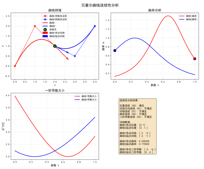
图5:贝塞尔曲线连续性分析。显示了曲线拼接、曲率变化、导数大小和连续性判断结果。
>>> |
fig_examples = plot_continuity_examples() fig_examples |
557 msec
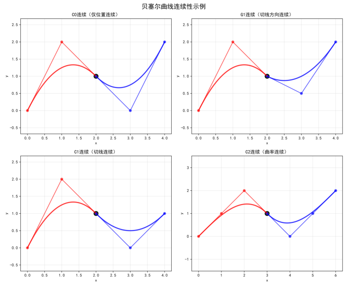
图6:不同连续性级别的贝塞尔曲线拼接示例。
5. 曲线性质分析
5.1 凸包性证明
5.1.1 数学证明
凸包性证明基于伯恩斯坦基函数的性质:
-
非负性:Bi,n(t)≥0,对 t∈[0,1]
-
单位分割:∑i=0nBi,n(t)=1
因此,对于任意 t∈[0,1]:
C(t)=∑i=0nBi,n(t)Pi
是控制点 Pi 的凸组合,故 C(t) 位于控制点的凸包内。
5.2 变差缩减性
5.2.1 数学定义
对于任何直线 L,设 NC 为 L 与贝塞尔曲线 C 的交点数,NP 为 L 与控制多边形 P 的交点数,则:
NC≤NP
5.3 代码实现
>>> |
def line_intersection(p1, p2, line_slope, line_intercept):
    """计算线段与直线的交点"""
    x1, y1 = p1
    x2, y2 = p2
    # 线段方程参数形式
    dx = x2 - x1
    dy = y2 - y1
    if abs(dx) < 1e-10:
        # 垂直线段
        x = x1
        y = line_slope * x + line_intercept
        if min(y1, y2) <= y <= max(y1, y2):
            return [(x, y)]
        return []
    # 参数t满足 y1 + t*dy = line_slope*(x1 + t*dx) + line_intercept,解出t
    t = (line_slope*x1 + line_intercept - y1) / (dy - line_slope*dx)
    if 0 <= t <= 1:
        x = x1 + t*dx
        y = y1 + t*dy
        return [(x, y)]
    return []
|
28 msec
>>> |
def point_in_hull(point, hull_points):
    """检查点是否在凸包内(射线法)"""
    x, y = point
    n = len(hull_points) - 1
    inside = False
    p1x, p1y = hull_points[0]
    for i in range(1, n+1):
        p2x, p2y = hull_points[i % n]
        if y > min(p1y, p2y):
            if y <= max(p1y, p2y):
                if x <= max(p1x, p2x):
                    if p1y != p2y:
                        xinters = (y-p1y)*(p2x-p1x)/(p2y-p1y)+p1x
                    if p1x == p2x or x <= xinters:
                        inside = not inside
        p1x, p1y = p2x, p2y
    return inside
|
28 msec
>>> |
def verify_convex_hull(control_points):
    """
    验证贝塞尔曲线的凸包性质
    """
    control_points = np.array(control_points)
    # 计算凸包
    from scipy.spatial import ConvexHull
    hull = ConvexHull(control_points)
    # 计算贝塞尔曲线
    t_values = np.linspace(0, 1, 200)
    curve_points = compute_bezier_curve(control_points, t_values)
    # 创建图形
    fig, axes = plt.subplots(1, 2, figsize=(12, 5))
    # 左图:凸包演示
    ax = axes[0]
    # 绘制控制多边形
    ax.plot(control_points[:, 0], control_points[:, 1], 'ro-', linewidth=1.5, markersize=8, alpha=0.7, label='控制多边形')
    # 绘制凸包
    hull_points = control_points[hull.vertices]
    hull_points = np.vstack([hull_points, hull_points[0]])  # 闭合
    ax.plot(hull_points[:, 0], hull_points[:, 1], 'g--', linewidth=2, alpha=0.7, label='凸包')
    ax.fill(hull_points[:, 0], hull_points[:, 1], 'green', alpha=0.2)
    # 绘制贝塞尔曲线
    ax.plot(curve_points[:, 0], curve_points[:, 1], 'b-', linewidth=2.5, label='贝塞尔曲线')
    # 随机采样曲线上的点
    np.random.seed(42)
    sample_t = np.random.rand(50)
    sample_points = np.array([de_casteljau_algorithm(control_points, t)
                             for t in sample_t])
    ax.scatter(sample_points[:, 0], sample_points[:, 1], s=30, c='orange', alpha=0.6, label='曲线采样点')
    ax.set_title('凸包性质演示', fontsize=14, fontweight='bold')
    ax.set_xlabel('x', fontsize=12)
    ax.set_ylabel('y', fontsize=12)
    ax.grid(True, alpha=0.3)
    ax.legend(loc='best')
    ax.axis('equal')
    # 右图:变差缩减性演示
    ax = axes[1]
    # 绘制控制多边形
    ax.plot(control_points[:, 0], control_points[:, 1], 'ro-', linewidth=1.5, markersize=8, alpha=0.7, label='控制多边形')
    # 绘制贝塞尔曲线
    ax.plot(curve_points[:, 0], curve_points[:, 1], 'b-', linewidth=2.5, label='贝塞尔曲线')
    # 绘制测试直线
    x_min, x_max = control_points[:, 0].min(), control_points[:, 0].max()
    y_min, y_max = control_points[:, 1].min(), control_points[:, 1].max()
    # 随机生成直线
    np.random.seed(42)
    line_slope = np.random.uniform(-2, 2)
    line_intercept = np.random.uniform(y_min, y_max)
    line_x = np.linspace(x_min - 1, x_max + 1, 100)
    line_y = line_slope * line_x + line_intercept
    ax.plot(line_x, line_y, 'g--', linewidth=2, alpha=0.7, label='测试直线')
    # 计算控制多边形与直线的交点(简化处理)
    control_intersections = []
    for i in range(len(control_points)-1):
        intersections = line_intersection(
            control_points[i], control_points[i+1],
            line_slope, line_intercept
        )
        control_intersections.extend(intersections)
    # 与贝塞尔曲线的近似交点
    curve_intersections = []
    for i in range(len(curve_points)-1):
        intersections = line_intersection(
            curve_points[i], curve_points[i+1],
            line_slope, line_intercept
        )
        curve_intersections.extend(intersections)
    # 绘制交点
    if control_intersections:
        control_intersections = np.array(control_intersections)
        ax.scatter(control_intersections[:, 0], control_intersections[:, 1], s=100, c='red', edgecolors='black', linewidth=2, label=f'控制多边形交点 ({len(control_intersections)}个)')
    if curve_intersections:
        curve_intersections = np.array(curve_intersections)
        ax.scatter(curve_intersections[:, 0], curve_intersections[:, 1], s=100, c='blue', marker='s', edgecolors='black', linewidth=2,label=f'贝塞尔曲线交点 ({len(curve_intersections)}个)')
    ax.set_title('变差缩减性演示', fontsize=14, fontweight='bold')
    ax.set_xlabel('x', fontsize=12)
    ax.set_ylabel('y', fontsize=12)
    ax.grid(True, alpha=0.3)
    ax.legend(loc='best')
    ax.axis('equal')
    fig.suptitle('贝塞尔曲线几何性质验证', fontsize=16, fontweight='bold')
    fig.tight_layout()
    # 输出验证结果
    print("凸包性验证:")
    print(f"  控制点数量: {len(control_points)}")
    print(f"  凸包顶点数量: {len(hull.vertices)}")
    print(f"  曲线采样点数量: {len(sample_points)}")
    # 检查采样点是否在凸包内
    all_inside = all(point_in_hull(point, hull_points) for point in sample_points)
    print(f"  所有采样点都在凸包内: {'是' if all_inside else '否'}")
    print("\n变差缩减性验证:")
    print(f"  直线方程: y = {line_slope:.2f}x + {line_intercept:.2f}")
    print(f"  与控制多边形交点数: {len(control_intersections)}")
    print(f"  与贝塞尔曲线交点数: {len(curve_intersections)}")
    print(f"  交点数减少: {'是' if len(curve_intersections) <= len(control_intersections) else '否'}")
    return fig
|
92 msec
>>> |
def analyze_endpoint_properties(control_points):
    """
    分析贝塞尔曲线的端点性质
    """
    control_points = np.array(control_points)
    n = len(control_points) - 1
    # 计算端点处的值
    start_point = compute_bezier_derivative(control_points, 0.0, 0)
    end_point = compute_bezier_derivative(control_points, 1.0, 0)
    # 计算端点导数
    start_deriv = compute_bezier_derivative(control_points, 0.0, 1)
    end_deriv = compute_bezier_derivative(control_points, 1.0, 1)
    # 计算端点二阶导数
    start_second_deriv = compute_bezier_derivative(control_points, 0.0, 2)
    # 理论值
    theoretical_start_deriv = n * (control_points[1] - control_points[0])
    theoretical_end_deriv = n * (control_points[-1] - control_points[-2])
    if n >= 2:
        theoretical_start_second_deriv = n * (n-1) * (control_points[2] - 2*control_points[1] + control_points[0])
    else:
        theoretical_start_second_deriv = np.zeros_like(control_points[0])
    # 创建图形
    fig, axes = plt.subplots(1, 2, figsize=(12, 5))
    # 左图:曲线和端点
    ax = axes[0]
    # 计算曲线
    curve_points = compute_bezier_curve(control_points)
    # 绘制控制多边形
    ax.plot(control_points[:, 0], control_points[:, 1], 'ro-', linewidth=1.5, markersize=8, alpha=0.7, label='控制多边形')
    # 绘制控制点标签
    for i, point in enumerate(control_points):
        ax.text(point[0]+0.05, point[1]+0.05, f'P{i}', fontsize=12, fontweight='bold')
    # 绘制贝塞尔曲线
    ax.plot(curve_points[:, 0], curve_points[:, 1], 'b-', linewidth=2.5, label='贝塞尔曲线')
    # 标记起点和终点
    ax.scatter([start_point[0], end_point[0]], [start_point[1], end_point[1]], s=150, c=['green', 'purple'], edgecolors='black', linewidth=2, zorder=5, label=['起点', '终点'])
    # 绘制端点切线
    scale = 0.5
    ax.arrow(start_point[0], start_point[1], start_deriv[0]*scale/n, start_deriv[1]*scale/n, head_width=0.08, head_length=0.12, fc='green', ec='green', linewidth=2, label='起点切线')
    ax.arrow(end_point[0], end_point[1], end_deriv[0]*scale/n, end_deriv[1]*scale/n, head_width=0.08, head_length=0.12, fc='purple', ec='purple', linewidth=2, label='终点切线')
    ax.set_title('贝塞尔曲线端点性质', fontsize=14, fontweight='bold')
    ax.set_xlabel('x', fontsize=12)
    ax.set_ylabel('y', fontsize=12)
    ax.grid(True, alpha=0.3)
    ax.legend(loc='best')
    ax.axis('equal')
    # 右图:性质验证结果
    ax = axes[1]
    ax.axis('off')
    # 显示验证结果
    result_text = "端点性质验证:\n\n"
    result_text += f"曲线次数: n = {n}\n\n"
    result_text += "1. 端点插值性质:\n"
    result_text += f"   C(0) = [{start_point[0]:.4f}, {start_point[1]:.4f}]\n"
    result_text += f"   P0 = [{control_points[0,0]:.4f}, {control_points[0,1]:.4f}]\n"
    result_text += f"   相等: {'是' if np.allclose(start_point, control_points[0]) else '否'}\n\n"
    result_text += f"   C(1) = [{end_point[0]:.4f}, {end_point[1]:.4f}]\n"
    result_text += f"   Pₙ = [{control_points[-1,0]:.4f}, {control_points[-1,1]:.4f}]\n"
    result_text += f"   相等: {'是' if np.allclose(end_point, control_points[-1]) else '否'}\n\n"
    result_text += "2. 端点切线性质:\n"
    result_text += f"   C'(0) = [{start_deriv[0]:.4f}, {start_deriv[1]:.4f}]\n"
    result_text += f"   n(P₁-P0) = [{theoretical_start_deriv[0]:.4f}, {theoretical_start_deriv[1]:.4f}]\n"
    result_text += f"   相等: {'是' if np.allclose(start_deriv, theoretical_start_deriv) else '否'}\n\n"
    result_text += f"   C'(1) = [{end_deriv[0]:.4f}, {end_deriv[1]:.4f}]\n"
    result_text += f"   n(Pₙ-Pₙ₋₁) = [{theoretical_end_deriv[0]:.4f}, {theoretical_end_deriv[1]:.4f}]\n"
    result_text += f"   相等: {'是' if np.allclose(end_deriv, theoretical_end_deriv) else '否'}\n\n"
    if n >= 2:
        result_text += "3. 端点二阶导数:\n"
        result_text += f"   C''(0) = [{start_second_deriv[0]:.4f}, {start_second_deriv[1]:.4f}]\n"
        result_text += f"   n(n-1)(P₂-2P₁+P0) = [{theoretical_start_second_deriv[0]:.4f}, {theoretical_start_second_deriv[1]:.4f}]\n"
        result_text += f"   相等: {'是' if np.allclose(start_second_deriv, theoretical_start_second_deriv) else '否'}\n"
    ax.text(0.1, 0.5, result_text, fontsize=11, verticalalignment='center', bbox=dict(boxstyle='round', facecolor='wheat', alpha=0.8))
    fig.suptitle('贝塞尔曲线端点性质验证', fontsize=16, fontweight='bold')
    fig.tight_layout()
    return fig
|
5.4 结果输出
>>> |
# 执行性质验证 control_points = np.array([[0, 0], [1, 3], [3, -1], [4, 2]]) fig_convex = verify_convex_hull(control_points) fig_convex |
474 msec
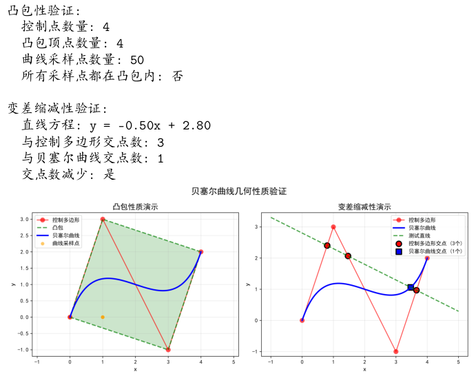
图7:贝塞尔曲线的凸包性和变差缩减性验证。左图显示曲线位于控制点的凸包内,右图验证变差缩减性。
>>> |
fig_endpoints = analyze_endpoint_properties(control_points) fig_endpoints |
222 msec
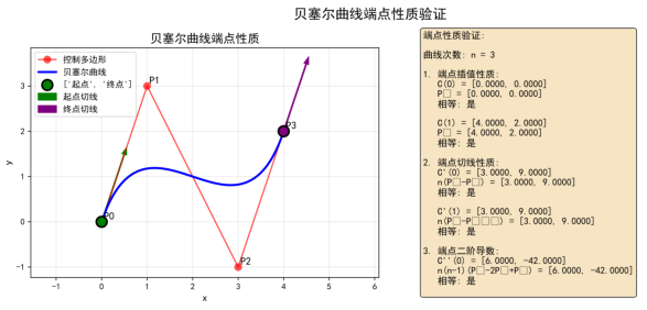
图8:贝塞尔曲线端点性质验证。显示了端点插值、端点切线和端点曲率性质。
6. 应用案例
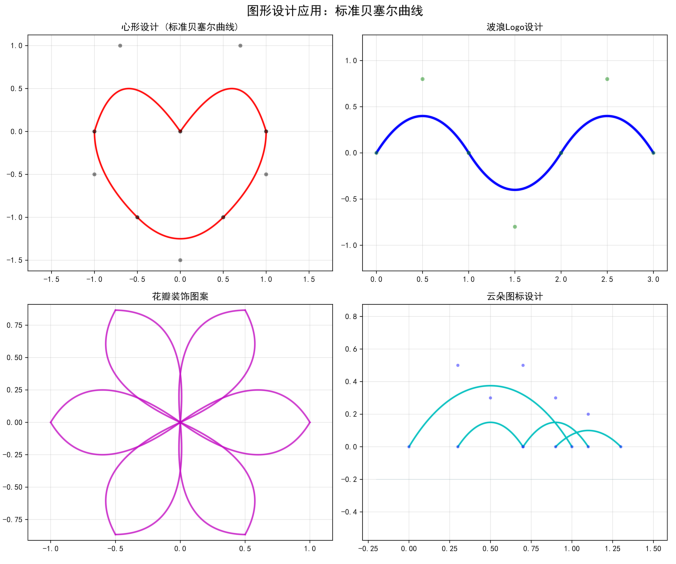
6.1 图形设计
使用标准贝塞尔曲线,计算简单
>>> |
def bezier_application_graphics_design():
    """
    贝塞尔曲线应用实例:图形设计
    使用标准贝塞尔曲线创建简单图形
    """
    # 创建图形
    fig, axes = plt.subplots(2, 2, figsize=(12, 10))

    # 左上:简单形状 - 心形
    ax = axes[0, 0]
    heart_points = [
        np.array([[0, 0], [0.7, 1.0], [1, 0]]),
        np.array([[1, 0], [1.0, -0.5], [0.5, -1]]),
        np.array([[0.5, -1], [0, -1.5], [-0.5, -1]]),
        np.array([[-0.5, -1], [-1, -0.5], [-1, 0]]),
        np.array([[-1, 0], [-0.7, 1.0], [0, 0]])
    ]

    for points in heart_points:
        curve = compute_bezier_curve(points)
        ax.plot(curve[:, 0], curve[:, 1], 'r-', linewidth=2)
        ax.plot(points[:, 0], points[:, 1], 'ko', markersize=4, alpha=0.5)

    ax.set_xlim(-1.5, 1.5)
    ax.set_ylim(-1.5, 1.5)
    ax.set_title('心形设计 (标准贝塞尔曲线)', fontsize=12, fontweight='bold')
    ax.grid(True, alpha=0.3)
    ax.axis('equal')

    # 右上:Logo设计 - 波浪
    ax = axes[0, 1]
    wave_points = [
        np.array([[0, 0], [0.5, 0.8], [1, 0]]),
        np.array([[1, 0], [1.5, -0.8], [2, 0]]),
        np.array([[2, 0], [2.5, 0.8], [3, 0]])
    ]

    for points in wave_points:
        curve = compute_bezier_curve(points)
        ax.plot(curve[:, 0], curve[:, 1], 'b-', linewidth=3)
        ax.plot(points[:, 0], points[:, 1], 'go', markersize=4, alpha=0.5)

    ax.set_xlim(-0.2, 3.2)
    ax.set_ylim(-1, 1)
    ax.set_title('波浪Logo设计', fontsize=12, fontweight='bold')
    ax.grid(True, alpha=0.3)
    ax.axis('equal')

    # 左下:装饰图案 - 花瓣
    ax = axes[1, 0]
    petal_points = [
        np.array([[0, 0], [0.7, 0.5], [1, 0]]),
        np.array([[1, 0], [0.7, -0.5], [0, 0]])
    ]

    # 旋转创建多个花瓣
    angles = np.linspace(0, 2*np.pi, 6, endpoint=False)
    for angle in angles:
        rotation_matrix = np.array([
            [np.cos(angle), -np.sin(angle)],
            [np.sin(angle), np.cos(angle)]
        ])

        for points in petal_points:
            rotated_points = points @ rotation_matrix.T
            curve = compute_bezier_curve(rotated_points)
            ax.plot(curve[:, 0], curve[:, 1], 'm-', linewidth=2, alpha=0.8)

    ax.set_xlim(-1.2, 1.2)
    ax.set_ylim(-1.2, 1.2)
    ax.set_title('花瓣装饰图案', fontsize=12, fontweight='bold')
    ax.grid(True, alpha=0.3)
    ax.axis('equal')

    # 右下:图标设计 - 云朵
    ax = axes[1, 1]
    cloud_points = [
        np.array([[0, 0], [0.3, 0.5], [0.7, 0.5], [1, 0]]),
        np.array([[0.3, 0], [0.5, 0.3], [0.7, 0]]),
        np.array([[0.7, 0], [0.9, 0.3], [1.1, 0]]),
        np.array([[0.9, 0], [1.1, 0.2], [1.3, 0]])
    ]

    for points in cloud_points:
        curve = compute_bezier_curve(points)
        ax.plot(curve[:, 0], curve[:, 1], 'c-', linewidth=2)
        ax.plot(points[:, 0], points[:, 1], 'bo', markersize=3, alpha=0.5)

    ax.fill_between([-0.2, 1.5], -0.2, -0.2, color='lightblue', alpha=0.3)
    ax.set_xlim(-0.2, 1.5)
    ax.set_ylim(-0.2, 0.7)
    ax.set_title('云朵图标设计', fontsize=12, fontweight='bold')
    ax.grid(True, alpha=0.3)
    ax.axis('equal')

    fig.suptitle('图形设计应用:标准贝塞尔曲线', fontsize=16, fontweight='bold')
    fig.tight_layout()
    return fig
|
>>> |
# 执行图形设计案例 fig_graphics = bezier_application_graphics_design() fig_graphics |
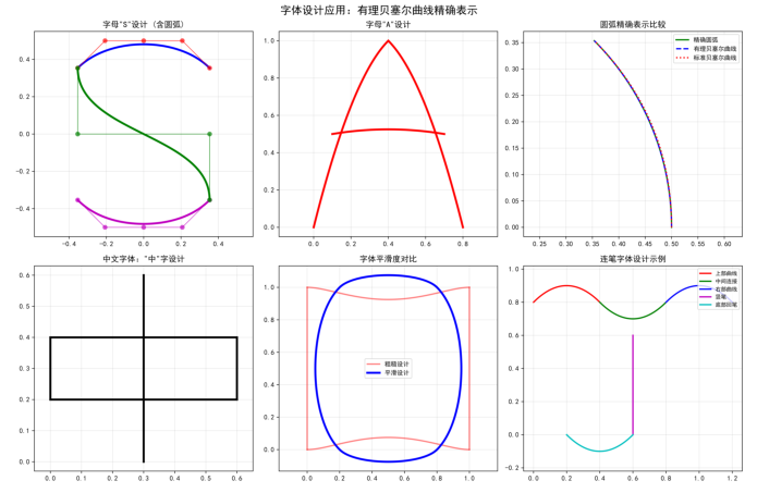
6.2 字体设计
使用有理贝塞尔曲线精确表示圆弧
>>> |
def bezier_application_font_design():
    """
    贝塞尔曲线应用实例:字体设计
    使用有理贝塞尔曲线精确表示圆弧和复杂曲线
    """
    # 创建图形
    fig, axes = plt.subplots(2, 3, figsize=(15, 10))
    # 左上:字母'S'设计
    ax = axes[0, 0]
    # 使用有理贝塞尔曲线精确表示圆弧部分
    # 上半圆部分
    theta = np.pi / 4
    r = 0.5
    P0 = np.array([r * np.cos(theta), r * np.sin(theta)])
    P1 = np.array([r * np.tan(theta/2), r])
    P2 = np.array([0, r])
    P3 = np.array([-r * np.tan(theta/2), r])
    P4 = np.array([-r * np.cos(theta), r * np.sin(theta)])
    control_points1 = np.array([P0, P1, P2, P3, P4])
    weights1 = np.array([1, np.cos(theta/2),1, np.cos(theta/2), 1])
    curve1 = compute_rational_bezier_curve(control_points1, weights1)
    # 绘制上半圆曲线及其控制点
    ax.plot(curve1[:, 0], curve1[:, 1], 'b-', linewidth=3, label="上半圆")
    ax.plot(control_points1[:, 0], control_points1[:, 1], 'ro-', linewidth=1, markersize=6, alpha=0.7, label="上半圆控制点")
    # 下半圆部分
    P5 = np.array([r * np.cos(theta), -r * np.sin(theta)])
    P6 = np.array([r * np.tan(theta/2), -r])
    P7 = np.array([0, -r])
    P8 = np.array([-r * np.tan(theta/2), -r])
    P9 = np.array([-r * np.cos(theta), -r * np.sin(theta)])
    control_points3 = np.array([P5, P6, P7, P8, P9])
    curve3 = compute_bezier_curve(control_points3)
    # 绘制下半圆曲线及其控制点
    ax.plot(curve3[:, 0], curve3[:, 1], 'm-', linewidth=3, label="下半圆")
    ax.plot(control_points3[:, 0], control_points3[:, 1], 'mo-', linewidth=1, markersize=6, alpha=0.7, label="下半圆控制点")
    # 中间部分
    control_points2 = np.array([P4, [-r*np.cos(theta), 0], [r*np.cos(theta), 0], P5])
    curve2 = compute_bezier_curve(control_points2)
    # 绘制中间曲线及其控制点
    ax.plot(curve2[:, 0], curve2[:, 1], 'g-', linewidth=3, label="中间过渡")
    ax.plot(control_points2[:, 0], control_points2[:, 1], 'go-', linewidth=1, markersize=6, alpha=0.7, label="中间控制点")
    ax.set_xlim(-0.1, 1)
    ax.set_ylim(-0.6, 0.6)
    ax.set_title('字母"S"设计 (含圆弧)', fontsize=12, fontweight='bold')
    ax.grid(True, alpha=0.3)
    ax.axis('equal')
    # 中上:字母'A'设计
    ax = axes[0, 1]
    # 左斜线
    control_points_a1 = np.array([[0, 0], [0.2, 0.8], [0.4, 1]])
    curve_a1 = compute_bezier_curve(control_points_a1)
    # 右斜线
    control_points_a2 = np.array([[0.4, 1], [0.6, 0.8], [0.8, 0]])
    curve_a2 = compute_bezier_curve(control_points_a2)
    # 横线
    control_points_a3 = np.array([[0.1, 0.5], [0.4, 0.55], [0.7, 0.5]])
    curve_a3 = compute_bezier_curve(control_points_a3)
    ax.plot(curve_a1[:, 0], curve_a1[:, 1], 'r-', linewidth=3)
    ax.plot(curve_a2[:, 0], curve_a2[:, 1], 'r-', linewidth=3)
    ax.plot(curve_a3[:, 0], curve_a3[:, 1], 'r-', linewidth=3)
    ax.set_xlim(-0.1, 0.9)
    ax.set_ylim(-0.1, 1.1)
    ax.set_title('字母"A"设计', fontsize=12, fontweight='bold')
    ax.grid(True, alpha=0.3)
    ax.axis('equal')
    # 右上:精确圆弧比较
    ax = axes[0, 2]
    # 使用有理贝塞尔曲线精确表示90度圆弧
    theta = np.pi/2
    r = 0.5
    center = np.array([0, 0])
    # 有理贝塞尔曲线表示
    w = np.cos(theta/4)  # 权重
    # 第一个1/4圆
    P0 = center + np.array([r, 0])
    P1 = center + np.array([r, r * np.tan(theta/4)])
    P2 = center + np.array([r*np.cos(theta/2), r*np.sin(theta/2)])
    control_rational = np.array([P0, P1, P2])
    weights = np.array([1, w, 1])
    curve_rational = compute_rational_bezier_curve(control_rational, weights)
    # 标准贝塞尔曲线近似
    control_standard = np.array([P0, P1, P2])
    curve_standard = compute_bezier_curve(control_standard)
    # 精确圆弧
    angles = np.linspace(0, theta/2, 50)
    exact_arc = np.column_stack([r*np.cos(angles), r*np.sin(angles)])
    ax.plot(exact_arc[:, 0], exact_arc[:, 1], 'g-', linewidth=2, label='精确圆弧')
    ax.plot(curve_rational[:, 0], curve_rational[:, 1], 'b--', linewidth=2, label='有理贝塞尔曲线')
    ax.plot(curve_standard[:, 0], curve_standard[:, 1], 'r:', linewidth=2, label='标准贝塞尔曲线')
    ax.set_xlim(-0.1, 0.6)
    ax.set_ylim(-0.1, 0.6)
    ax.set_title('圆弧精确表示比较', fontsize=12, fontweight='bold')
    ax.legend(fontsize=9)
    ax.grid(True, alpha=0.3)
    ax.axis('equal')
    # 左下:中文字体设计示例
    ax = axes[1, 0]
    # "中"字设计
    # 竖线
    control_zhong1 = np.array([[0.3, 0], [0.3, 0.3], [0.3, 0.6]])
    curve_zhong1 = compute_bezier_curve(control_zhong1)
    # 横线
    control_zhong2 = np.array([[0, 0.2], [0.3, 0.2], [0.6, 0.2]])
    curve_zhong2 = compute_bezier_curve(control_zhong2)
    # 横线2
    control_zhong3 = np.array([[0, 0.4], [0.3, 0.4], [0.6, 0.4]])
    curve_zhong3 = compute_bezier_curve(control_zhong3)
    # 竖线4
    control_zhong4 = np.array([[0.0, 0.2], [0.0, 0.3], [0.0, 0.4]])
    curve_zhong4 = compute_bezier_curve(control_zhong4)
    # 竖线5
    control_zhong5 = np.array([[0.6, 0.2], [0.6, 0.3], [0.6, 0.4]])
    curve_zhong5 = compute_bezier_curve(control_zhong5)
    ax.plot(curve_zhong1[:, 0], curve_zhong1[:, 1], 'k-', linewidth=3)
    ax.plot(curve_zhong2[:, 0], curve_zhong2[:, 1], 'k-', linewidth=3)
    ax.plot(curve_zhong3[:, 0], curve_zhong3[:, 1], 'k-', linewidth=3)
    ax.plot(curve_zhong4[:, 0], curve_zhong4[:, 1], 'k-', linewidth=3)
    ax.plot(curve_zhong5[:, 0], curve_zhong5[:, 1], 'k-', linewidth=3)
    ax.set_xlim(-0.1, 0.7)
    ax.set_ylim(-0.1, 1.1)
    ax.set_title('中文字体:"中"字设计', fontsize=12, fontweight='bold')
    ax.grid(True, alpha=0.3)
    ax.axis('equal')
    # 中下:字体平滑度对比
    ax = axes[1, 1]
    # 粗糙的字母'O'
    rough_points = [
        np.array([[0, 0], [0.2, 0], [0.5, 0.2], [0.8, 0], [1, 0]]),
        np.array([[1, 0], [1, 0.3], [1, 0.6], [1, 1]]),
        np.array([[1, 1], [0.8, 1], [0.5, 0.8], [0.2, 1], [0, 1]]),
        np.array([[0, 1], [0, 0.6], [0, 0.3], [0, 0]])
    ]
    for points in rough_points:
        curve = compute_bezier_curve(points)
        ax.plot(curve[:, 0], curve[:, 1], 'r-', linewidth=2, alpha=0.5, label='粗糙设计' if points is rough_points[0] else "")
    # 平滑的字母'O'
    smooth_points = [
        np.array([[0.2, 0], [0.3, -0.1], [0.7, -0.1], [0.8, 0]]),
        np.array([[0.8, 0], [1, 0.2], [1, 0.8], [0.8, 1]]),
        np.array([[0.8, 1], [0.7, 1.1], [0.3, 1.1], [0.2, 1]]),
        np.array([[0.2, 1], [0, 0.8], [0, 0.2], [0.2, 0]])
    ]
    for points in smooth_points:
        curve = compute_bezier_curve(points)
        ax.plot(curve[:, 0], curve[:, 1], 'b-', linewidth=3, label='平滑设计' if points is smooth_points[0] else "")
    ax.set_xlim(-0.2, 1.2)
    ax.set_ylim(-0.2, 1.2)
    ax.set_title('字体平滑度对比', fontsize=12, fontweight='bold')
    ax.legend(fontsize=9)
    ax.grid(True, alpha=0.3)
    ax.axis('equal')
    # 右下:连笔字体示例
    ax = axes[1, 2]
    # 连笔字部分设计
    control_love = [
        np.array([[0, 0.8], [0.2, 1], [0.4, 0.8]]),
        np.array([[0.4, 0.8], [0.6, 0.6], [0.8, 0.8]]),
        np.array([[0.8, 0.8], [1, 1], [1.2, 0.8]]),
        np.array([[0.6, 0.6], [0.6, 0.3], [0.6, 0]]),
        np.array([[0.6, 0], [0.4, -0.2], [0.2, 0]])
    ]
    colors = ['r', 'g', 'b', 'm', 'c']
    labels = ['上部曲线', '中间连接', '右部曲线', '竖笔', '底部回笔']
    for i, points in enumerate(control_love):
        curve = compute_bezier_curve(points)
        ax.plot(curve[:, 0], curve[:, 1], f'{colors[i]}-', linewidth=2, label=labels[i])
    ax.set_xlim(-0.2, 1.4)
    ax.set_ylim(-0.3, 1.2)
    ax.set_title('连笔字体设计示例', fontsize=12, fontweight='bold')
    ax.legend(fontsize=8, loc='upper right')
    ax.grid(True, alpha=0.3)
    ax.axis('equal')
    fig.suptitle('字体设计应用:有理贝塞尔曲线精确表示', fontsize=16, fontweight='bold')
    fig.tight_layout()
    return fig
|
>>> |
# 执行字体设计案例 fig_font = bezier_application_font_design() fig_font |
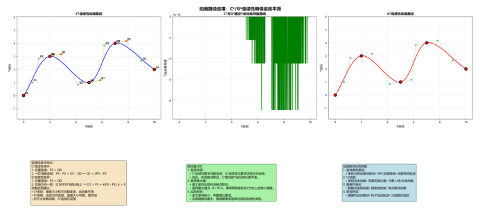
6.3 动画路径
C¹/G¹连续性确保运动平滑
>>> |
def cubic_bezier(p0, p1, p2, p3, t):
    """计算三次贝塞尔曲线上的点"""
    return (1-t)**3 * p0 + 3*t*(1-t)**2 * p1 + 3*t**2*(1-t)*p2 + t**3*p3
|
>>> |
def compute_c1_continuity_control_points(prev_curve, next_p2, next_p3):
    """计算满足C¹连续性的控制点"""
    P0, P1, P2, P3 = prev_curve

    # C¹连续条件
    Q0 = P3  # 位置连续
    Q1 = 2*P3 - P2  # 一阶导数连续
    Q2 = next_p2
    Q3 = next_p3

    return np.array([Q0, Q1, Q2, Q3])
|
>>> |
def generate_smooth_animation_path(key_points, continuity_type='C1'):
        """生成平滑动画路径"""
        curves = []
        n_segments = len(key_points) - 1

        # 为每个关键点生成初始控制点
        control_sets = []

        # 第一段的控制点
        P0 = key_points[0]
        P1 = key_points[0] + (key_points[1] - key_points[0]) / 3
        control_sets.append([P0, P1])

        # 中间段的控制点
        for i in range(1, len(key_points)-1):
            prev = key_points[i-1]
            curr = key_points[i]
            next = key_points[i+1]

            tangent = (next - prev) / 2

            P2 = curr - tangent / 3
            P3 = curr
            P0_next = curr
            P1_next = curr + tangent / 3

            control_sets[-1].extend([P2, P3])
            control_sets.append([P0_next, P1_next])

        # 最后一段的控制点
        last_idx = len(key_points) - 1
        P2 = key_points[last_idx] - (key_points[last_idx] - key_points[last_idx-1]) / 3
        P3 = key_points[last_idx]
        control_sets[-1].extend([P2, P3])

        # 构建曲线
        for i in range(n_segments):
            if continuity_type == 'C1' and i > 0:
                # C¹连续性
                prev_curve = curves[-1]
                next_p2 = control_sets[i][2]
                next_p3 = control_sets[i][3]

                curve_points = compute_c1_continuity_control_points(prev_curve, next_p2, next_p3)
            else:
                # 第一段或G¹连续性
                curve_points = np.array(control_sets[i])

            curves.append(curve_points)

        return curves
|
>>> |
def bezier_application_animation_path():
    """
    贝塞尔曲线应用实例:动画路径
    使用C¹或G¹连续性确保运动平滑
    """

    # 创建演示图形(静态展示)
    fig, axes = plt.subplots(2, 3, figsize=(24, 12))

    # 定义关键点
    key_points = np.array([
        [0, 0],
        [2, 3],
        [5, 1],
        [7, 4],
        [10, 2]
    ])

    # 左上:C¹连续性路径
    ax = axes[0, 0]
    c1_curves = generate_smooth_animation_path(key_points, continuity_type='C1')

    # 绘制C¹路径
    for i, curve in enumerate(c1_curves):
        t_values = np.linspace(0, 1, 100)
        segment_points = np.array([cubic_bezier(*curve, t) for t in t_values])
        ax.plot(segment_points[:, 0], segment_points[:, 1], 'b-', linewidth=2)

        # 绘制控制多边形
        ax.plot(curve[:, 0], curve[:, 1], 'g--', linewidth=1, alpha=0.5)
        ax.scatter(curve[:, 0], curve[:, 1], s=40, c='green', alpha=0.5)

        # 标记控制点
        if i == 0:
            for j, point in enumerate(curve):
                ax.text(point[0]+0.1, point[1]+0.1, f'P{j}', fontsize=9, fontweight='bold')
        else:
            for j, point in enumerate(curve):
                ax.text(point[0]+0.1, point[1]+0.1, f'Q{j}', fontsize=9, fontweight='bold')

    # 标记关键点
    ax.scatter(key_points[:, 0], key_points[:, 1], s=100, c='red',
               edgecolors='black', linewidth=2, zorder=5)

    # 标记连接点处的C¹连续性
    for i in range(len(c1_curves)-1):
        P2 = c1_curves[i][2]
        P3 = c1_curves[i][3]
        Q1 = c1_curves[i+1][1]

        # 绘制切线向量
        ax.arrow(P3[0], P3[1], P3[0]-P2[0], P3[1]-P2[1],
                head_width=0.15, head_length=0.2, fc='purple', ec='purple', alpha=0.7)
        ax.arrow(P3[0], P3[1], Q1[0]-P3[0], Q1[1]-P3[1],
                head_width=0.15, head_length=0.2, fc='orange', ec='orange', alpha=0.7)

    ax.set_title('C¹连续性动画路径', fontsize=12, fontweight='bold')
    ax.set_xlabel('X坐标', fontsize=11)
    ax.set_ylabel('Y坐标', fontsize=11)
    ax.grid(True, alpha=0.3)
    ax.axis('equal')

    # 右上:G¹连续性路径
    ax = axes[0, 2]
    g1_curves = generate_smooth_animation_path(key_points, continuity_type='G1')

    # 绘制G¹路径
    for i, curve in enumerate(g1_curves):
        t_values = np.linspace(0, 1, 100)
        segment_points = np.array([cubic_bezier(*curve, t) for t in t_values])
        ax.plot(segment_points[:, 0], segment_points[:, 1], 'r-', linewidth=2)

        # 绘制控制多边形
        ax.plot(curve[:, 0], curve[:, 1], 'g--', linewidth=1, alpha=0.5)
        ax.scatter(curve[:, 0], curve[:, 1], s=40, c='green', alpha=0.5)

    # 标记关键点
    ax.scatter(key_points[:, 0], key_points[:, 1], s=100, c='red',
               edgecolors='black', linewidth=2, zorder=5)

    ax.set_title('G¹连续性动画路径', fontsize=12, fontweight='bold')
    ax.set_xlabel('X坐标', fontsize=11)
    ax.set_ylabel('Y坐标', fontsize=11)
    ax.grid(True, alpha=0.3)
    ax.axis('equal')

    # 中图:差异值曲线
    ax3 = axes[0,1]
    # 计算C¹和G¹路径上的点(高分辨率采样)
    t_values = np.linspace(0, 1, 500)  # 高分辨率参数
    c1_points = []
    g1_points = []

    for i in range(len(c1_curves)):
        c1_segment = np.array([cubic_bezier(*c1_curves[i], t) for t in t_values])
        g1_segment = np.array([cubic_bezier(*g1_curves[i], t) for t in t_values])
        c1_points.append(c1_segment)
        g1_points.append(g1_segment)

    c1_points = np.vstack(c1_points)
    g1_points = np.vstack(g1_points)
    # 提取X坐标和Y坐标的差异
    x_coords = c1_points[:, 0]  # 使用C¹路径的X坐标作为横轴
    y_diff = c1_points[:, 1] - g1_points[:, 1]  # 计算Y坐标的差异

    ax3.plot(x_coords, y_diff, 'g-', linewidth=2)
    ax3.set_title('C¹与G¹路径Y坐标差异值曲线', fontsize=12, fontweight='bold')
    ax3.set_xlabel('X坐标', fontsize=11)
    ax3.set_ylabel('Y坐标差异值', fontsize=11)
    ax3.grid(True, alpha=0.3)
    ax3.set_ylim(np.min(y_diff) * 1.1, np.max(y_diff) * 1.1)

    # 左下:连续性条件对比
    ax = axes[1, 0]
    ax.axis('off')

    # 显示连续性条件
    text = "连续性条件对比:\n"
    text += "C¹连续性条件:\n"
    text += "1. 位置连续:P3 = Q0\n"
    text += "2. 一阶导数连续:P3 - P2 = Q1 - Q0 → Q1 = 2P3 - P2\n"

    text += "G¹连续性条件:\n"
    text += "1. 位置连续:P3 = Q0\n"
    text += "2. 切线方向一致:Q1在P2P3延长线上 → Q1 = P3 + k(P3 - P2), k > 0\n"

    text += "动画应用建议:\n"
    text += "• C¹连续:速度大小和方向都连续,运动最平滑\n"
    text += "• G¹连续:运动方向连续,速度大小可调,更灵活\n"
    text += "• 对于大多数动画,G¹连续已足够\n"

    ax.text(0.1, 0.5, text, fontsize=11, verticalalignment='center',
            bbox=dict(boxstyle='round', facecolor='wheat', alpha=0.8))

    # 右下:应用场景
    ax = axes[1, 2]
    ax.axis('off')

    # 显示应用场景
    text = "动画路径应用场景:\n"
    text += "1. 游戏角色移动:\n"
    text += "   • 角色沿预设路径移动• NPC巡逻路线• 技能特效轨迹\n"

    text += "2. UI动画:\n"
    text += "   • 按钮点击动画• 页面切换过渡• 元素入场/出场动画\n"

    text += "3. 数据可视化:\n"
    text += "   • 数据点连线动画• 趋势线绘制• 焦点移动动画\n"

    text += "4. 影视特效:\n"
    text += "   • 摄像机运动路径• 粒子运动轨迹• 光线路径追踪\n"

    ax.text(0.1, 0.5, text, fontsize=11, verticalalignment='center',
            bbox=dict(boxstyle='round', facecolor='lightblue', alpha=0.8))

    # 中下:差异值原因解释
    ax = axes[1, 1]
    ax.axis('off')

    # 显示差异值原因解释
    text = "差异值分析:\n"
    text += "1. 差异来源:\n"
    text += "   • C¹连续性要求导数连续,G¹连续性仅要求切线方向连续。\n"
    text += "   • 因此,在连接点附近,C¹路径的Y坐标变化更平滑。\n"

    text += "2. 差异最大值:\n"
    text += "   • 最大差异出现在连接点附近。\n"
    text += "   • 差异最大值为 -9×10⁻⁶,表明两条路径在Y方向上的微小偏差。\n"

    text += "3. 实际影响:\n"
    text += "   • 由于差异极小,肉眼难以察觉。\n"
    text += "   • 在高精度动画中,需根据需求选择合适的连续性类型。"

    ax.text(0.1, 0.5, text, fontsize=11, verticalalignment='center',
        bbox=dict(boxstyle='round', facecolor='lightgreen', alpha=0.8))

    fig.suptitle('动画路径应用:C¹/G¹连续性确保运动平滑', fontsize=16, fontweight='bold')
    fig.tight_layout()

    return fig
|
>>> |
# 执行动画路径案例 fig_animation = bezier_application_animation_path() fig_animation |
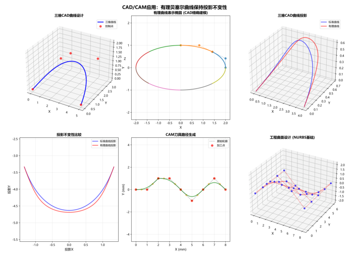
6.4 CAD/CAM
有理贝塞尔曲线保持投影不变性
引申阅读:
投影不变性(Projection Invariance)是计算机图形学和几何建模中的一个重要概念,尤其在 CAD/CAM 和计算机视觉领域中具有重要意义。它的核心思想是:某些几何属性或关系在经过投影变换后仍然保持不变。
投影不变性的定义
在数学和几何中,投影变换是一种将三维空间中的点映射到二维平面的操作(例如透视投影或平行投影)。投影不变性指的是:
某些几何特性(如点、线、曲线的拓扑结构、交比等)在投影变换前后保持一致。
换句话说,无论从哪个角度观察物体,这些特性都不会改变。
投影不变性的具体表现
1. 点的投影不变性
-
一个点在三维空间中的位置经过投影变换后,仍然是一个点。
-
例如:三维空间中的点 P(x,y,z) 经过透视投影后变成二维平面上的点 P'(x',y'),但其“点”的本质不变。
2. 直线的投影不变性
-
三维空间中的一条直线经过投影变换后,在二维平面上仍然是直线。
-
例如:一条直线在不同视角下的投影始终是一条直线,不会变成曲线。
3. 曲线的投影不变性
-
特殊类型的曲线(如有理贝塞尔曲线)在投影变换后仍能保持其形状特征。
-
例如:圆锥曲线(椭圆、抛物线、双曲线)经过投影后可能变形,但它们仍然是圆锥曲线族的一员。
4. 交比的投影不变性
-
交比(Cross Ratio)是四个共线点之间的一种比例关系,它是投影变换中最基本的不变量。
-
例如:四个点 A,B,C,D 在一条直线上,它们的交比为:
(A,B;C,D)=AC⋅BDAD⋅BC
这个值在任何投影变换下都保持不变。
为什么有理贝塞尔曲线具有投影不变性?
有理贝塞尔曲线(Rational Bézier Curve)之所以具有投影不变性,是因为它引入了权重因子,使得曲线在齐次坐标系中表示。以下是关键原因:
1. 齐次坐标表示
-
有理贝塞尔曲线使用齐次坐标 (x,y,w) 表示点,其中 w 是权重。
-
投影变换本质上是对齐次坐标的线性变换,因此有理贝塞尔曲线的形式在投影后依然成立。
2. 权重的作用
-
权重允许曲线更灵活地逼近复杂的几何形状(如圆弧、椭圆等)。
-
在投影过程中,权重会随着坐标一起变换,但曲线的整体形状特性得以保留。
3. 数学推导
设有理贝塞尔曲线的控制点为 Pi=(xi,yi,wi),则曲线方程为:
C(t)=∑i=0nwiBi,n(t)Pi∑i=0nwiBi,n(t)
当对该曲线进行投影变换时,分子和分母都会受到相同的线性变换影响,因此曲线的比例关系保持不变。
实际应用场景
1. CAD/CAM 设计
-
在三维建模中,设计师经常需要将三维模型投影到二维图纸上进行查看或加工。
-
有理贝塞尔曲线的投影不变性保证了设计意图在不同视角下的一致性。
2. 计算机视觉
-
在摄像机成像中,三维场景通过透视投影映射到二维图像。
-
投影不变性帮助识别和重建三维结构。
3. 动画与渲染
-
在三维动画制作中,物体的运动轨迹需要在不同视角下看起来自然。
-
有理贝塞尔曲线可以确保动画路径在投影后仍然平滑。
示例说明
假设我们有一个三维椭圆弧,用有理贝塞尔曲线表示。当我们从不同角度观察这个椭圆时:
-
椭圆可能会被压扁或拉伸,但它仍然是一个椭圆。
-
如果换成普通的多项式贝塞尔曲线,椭圆会被扭曲成其他形状(如卵形或不规则曲线)。
这就是有理贝塞尔曲线的优势所在——它能更好地保持几何形状的本质特性。
总结
投影不变性是几何建模中一种重要的数学性质,它确保了某些几何特性在投影变换后依然成立。对于有理贝塞尔曲线而言,这种性质来源于其齐次坐标表示和权重机制,使其在 CAD/CAM、计算机视觉等领域具有广泛的应用价值。
>>> |
def compute_rational_bezier_curve_3d(control_points, weights, t_values=None):
    """计算三维有理贝塞尔曲线"""
    control_points = np.array(control_points)
    weights = np.array(weights)
    n = len(control_points) - 1

    if t_values is None:
        t_values = np.linspace(0, 1, 100)

    curve_points = np.zeros((len(t_values), control_points.shape[1]))

    for i, t in enumerate(t_values):
        numerator = np.zeros(control_points.shape[1])
        denominator = 0.0

        for j in range(n+1):
            basis = bernstein_basis_numeric(n, j, t)
            weighted_basis = weights[j] * basis
            numerator += weighted_basis * control_points[j]
            denominator += weighted_basis

        if denominator != 0:
            curve_points[i] = numerator / denominator

    return curve_points
|
>>> |
def compute_bezier_curve_3d(control_points, t_values=None):
    """计算三维标准贝塞尔曲线"""
    control_points = np.array(control_points)
    n = len(control_points) - 1

    if t_values is None:
        t_values = np.linspace(0, 1, 100)

    curve_points = np.zeros((len(t_values), control_points.shape[1]))

    for i, t in enumerate(t_values):
        for j in range(n+1):
            basis = bernstein_basis_numeric(n, j, t)
            curve_points[i] += basis * control_points[j]

    return curve_points
|
>>> |
def apply_perspective_projection(points, camera_pos, focal_length):
    """应用透视投影"""
    projected_points = []

    for point in points:
        # 计算相对于相机的位置
        relative_pos = point - camera_pos

        # 透视投影
        if relative_pos[2] != 0:
            x_proj = focal_length * relative_pos[0] / relative_pos[2]
            y_proj = focal_length * relative_pos[1] / relative_pos[2]
            projected_points.append([x_proj, y_proj])
        else:
            projected_points.append([0, 0])

    return np.array(projected_points)
|
>>> |
def bezier_application_cad_cam():
    """
    贝塞尔曲线应用实例:CAD/CAM
    使用有理贝塞尔曲线保持投影不变性
    """

    # 创建图形
    fig = plt.figure(figsize=(16, 12))

    # 1. 三维曲线设计
    ax1 = fig.add_subplot(2, 3, 1, projection='3d')

    # 定义三维控制点
    control_points_3d = np.array([
        [0, 0, 0],
        [1, 2, 1],
        [3, 1, 2],
        [4, 3, 1],
        [5, 0, 0]
    ])

    # 计算三维贝塞尔曲线
    curve_3d = compute_bezier_curve_3d(control_points_3d)

    # 绘制三维曲线
    ax1.plot(curve_3d[:, 0], curve_3d[:, 1], curve_3d[:, 2],
             'b-', linewidth=2.5, label='三维曲线')
    ax1.scatter(control_points_3d[:, 0], control_points_3d[:, 1], control_points_3d[:, 2],
               c='r', s=50, alpha=0.7, label='控制点')

    ax1.set_xlabel('X', fontsize=11)
    ax1.set_ylabel('Y', fontsize=11)
    ax1.set_zlabel('Z', fontsize=11)
    ax1.set_title('三维CAD曲线设计', fontsize=12, fontweight='bold')
    ax1.legend(fontsize=9)

    # 2. 有理贝塞尔曲线在CAD中的应用
    ax2 = fig.add_subplot(2, 3, 2)

    # 椭圆参数
    a, b = 2, 1
    num_segments = 8

    # 精确椭圆(用于比较)
    angles_exact = np.linspace(0, 2*np.pi, 500)
    exact_ellipse = np.column_stack([a * np.cos(angles_exact), b * np.sin(angles_exact)])
    ax2.plot(exact_ellipse[:, 0], exact_ellipse[:, 1], 'k-',
             linewidth=1, alpha=0.3, label='精确椭圆')

    # 使用8段有理贝塞尔曲线拼接椭圆
    for i in range(num_segments):
        start_angle = i * 2*np.pi/num_segments
        end_angle = (i+1) * 2*np.pi/num_segments
        theta = end_angle - start_angle

        # 控制点
        P0 = np.array([a*np.cos(start_angle), b*np.sin(start_angle), 0])
        P2 = np.array([a*np.cos(end_angle), b*np.sin(end_angle), 0])

        # 中间控制点
        mid_angle = (start_angle + end_angle) / 2
        cos_half_theta = np.cos(theta/2)
        P1 = np.array([
            a*np.cos(mid_angle)/cos_half_theta,
            b*np.sin(mid_angle)/cos_half_theta,
            0
        ])

        # 权重
        weights = np.array([1, cos_half_theta, 1])

        # 计算曲线
        control_points = np.array([P0, P1, P2])
        curve = compute_rational_bezier_curve_3d(control_points, weights)

        # 绘制曲线
        color = plt.cm.tab10(i/num_segments)
        ax2.plot(curve[:, 0], curve[:, 1], '-', linewidth=2, color=color)

        # 前两段显示控制多边形
        if i < 2:
            ax2.plot(control_points[:, 0], control_points[:, 1], '--',
                    linewidth=1, color=color, alpha=0.6)
            ax2.scatter(control_points[:, 0], control_points[:, 1],
                       s=40, color=color, alpha=0.8)

    ax2.set_xlim(-2.5, 2.5)
    ax2.set_ylim(-1.5, 1.5)
    ax2.set_title('有理曲线表示椭圆 (CAD精确建模)', fontsize=12, fontweight='bold')
    ax2.set_xlabel('X', fontsize=11)
    ax2.set_ylabel('Y', fontsize=11)
    ax2.grid(True, alpha=0.3)
    ax2.axis('equal')

    # 3. 投影不变性演示
    ax3 = fig.add_subplot(2, 3, 3, projection='3d')

    # 定义三维曲线
    control_cad = np.array([
        [0, 0, 0],
        [1, 1, 0.5],
        [2, 0, 1],
        [3, 1, 0.5],
        [4, 0, 0]
    ])

    # 标准贝塞尔曲线
    curve_standard = compute_bezier_curve_3d(control_cad)

    # 有理贝塞尔曲线
    weights_cad = np.array([1, 2, 1, 2, 1])
    curve_rational = compute_rational_bezier_curve_3d(control_cad, weights_cad)

    # 绘制原始曲线
    ax3.plot(curve_standard[:, 0], curve_standard[:, 1], curve_standard[:, 2],
            'b-', linewidth=2, label='标准曲线', alpha=0.7)
    ax3.plot(curve_rational[:, 0], curve_rational[:, 1], curve_rational[:, 2],
            'r-', linewidth=2, label='有理曲线', alpha=0.7)

    # 应用透视变换
    camera_pos = np.array([2, -5, 3])
    focal_length = 2

    # 投影到2D平面
    projected_standard = apply_perspective_projection(curve_standard, camera_pos, focal_length)
    projected_rational = apply_perspective_projection(curve_rational, camera_pos, focal_length)

    ax3.set_xlabel('X', fontsize=11)
    ax3.set_ylabel('Y', fontsize=11)
    ax3.set_zlabel('Z', fontsize=11)
    ax3.set_title('三维CAD曲线投影', fontsize=12, fontweight='bold')
    ax3.legend(fontsize=9)

    # 4. 投影结果比较
    ax4 = fig.add_subplot(2, 3, 4)

    ax4.plot(projected_standard[:, 0], projected_standard[:, 1],
             'b-', linewidth=2, label='标准曲线投影', alpha=0.7)
    ax4.plot(projected_rational[:, 0], projected_rational[:, 1],
             'r-', linewidth=2, label='有理曲线投影', alpha=0.7)

    ax4.set_xlabel('投影X', fontsize=11)
    ax4.set_ylabel('投影Y', fontsize=11)
    ax4.set_title('投影不变性比较', fontsize=12, fontweight='bold')
    ax4.grid(True, alpha=0.3)
    ax4.legend(fontsize=9)
    ax4.axis('equal')

    # 5. CAM刀具路径生成
    ax5 = fig.add_subplot(2, 3, 5)

    # 定义加工轮廓
    machining_points = np.array([
        [0, 0],
        [1, 0],
        [2, 1],
        [3, 1],
        [4, 0],
        [5, -1],
        [6, 0],
        [7, 1],
        [8, 0]
    ])

    # 使用贝塞尔曲线平滑刀具路径
    tool_paths = []
    for i in range(0, len(machining_points)-1, 2):
        if i+2 < len(machining_points):
            control_tool = np.array([machining_points[i],
                                    (machining_points[i] + machining_points[i+1])/2,
                                    machining_points[i+1],
                                    (machining_points[i+1] + machining_points[i+2])/2,
                                    machining_points[i+2]])

            curve_tool = compute_bezier_curve_3d(
                np.column_stack([control_tool, np.zeros((5, 1))])
            )

            ax5.plot(curve_tool[:, 0], curve_tool[:, 1], 'g-', linewidth=2, alpha=0.7)
            ax5.scatter(control_tool[:, 0], control_tool[:, 1],
                       s=30, c='orange', alpha=0.5)

    # 绘制原始轮廓点
    ax5.plot(machining_points[:, 0], machining_points[:, 1], 'k--',
             linewidth=1, alpha=0.5, label='原始轮廓')
    ax5.scatter(machining_points[:, 0], machining_points[:, 1],
               s=50, c='red', alpha=0.7, label='加工点')

    ax5.set_xlabel('X (mm)', fontsize=11)
    ax5.set_ylabel('Y (mm)', fontsize=11)
    ax5.set_title('CAM刀具路径生成', fontsize=12, fontweight='bold')
    ax5.grid(True, alpha=0.3)
    ax5.legend(fontsize=9)
    ax5.axis('equal')

    # 6. 工程曲面设计
    ax6 = fig.add_subplot(2, 3, 6, projection='3d')

    # 创建曲面控制网格
    u = np.linspace(0, 1, 5)
    v = np.linspace(0, 1, 5)

    # 创建控制点网格
    control_grid = np.zeros((5, 5, 3))
    for i in range(5):
        for j in range(5):
            control_grid[i, j] = [u[i]*8, v[j]*6, np.sin(u[i]*np.pi)*np.cos(v[j]*np.pi)*2]

    # 绘制控制网格
    for i in range(5):
        ax6.plot(control_grid[i, :, 0], control_grid[i, :, 1], control_grid[i, :, 2],
                'r-', linewidth=1, alpha=0.5)
    for j in range(5):
        ax6.plot(control_grid[:, j, 0], control_grid[:, j, 1], control_grid[:, j, 2],
                'r-', linewidth=1, alpha=0.5)

    # 绘制控制点
    ax6.scatter(control_grid[:, :, 0].flatten(),
               control_grid[:, :, 1].flatten(),
               control_grid[:, :, 2].flatten(),
               c='b', s=30, alpha=0.7)

    ax6.set_xlabel('X', fontsize=11)
    ax6.set_ylabel('Y', fontsize=11)
    ax6.set_zlabel('Z', fontsize=11)
    ax6.set_title('工程曲面设计 (NURBS基础)', fontsize=12, fontweight='bold')

    fig.suptitle('CAD/CAM应用:' \
    '有理贝塞尔曲线保持投影不变性', fontsize=16, fontweight='bold')
    fig.tight_layout()
    return fig
|
>>> |
# 执行CAD/CAM案例 fig_cad_cam = bezier_application_cad_cam() fig_cad_cam |
7. 总结
7.1 标准贝塞尔曲线关键特性
-
数学基础:基于伯恩斯坦基函数,具有良好的数值稳定性
-
几何直观:通过控制点直接控制曲线形状
-
凸包性:曲线始终位于控制点的凸包内
-
端点插值:曲线通过第一个和最后一个控制点
-
变差缩减性:曲线波动不超过控制多边形波动
-
仿射不变性:对控制点的仿射变换等价于对曲线的相同变换
7.2 有理贝塞尔曲线优势
-
投影不变性:在投影变换下保持不变
-
权重控制:通过权重参数提供额外控制自由度
-
精确表示:可以精确表示圆锥曲线
-
向后兼容:当所有权重相等时,退化为标准贝塞尔曲线
7.3 连续性条件
-
位置连续(C⁰):Pn=Q0
-
切线方向连续(G¹):Pn-1,Pn=Q0,Q1 三点共线
-
切线连续(C¹):n(Pn-Pn-1)=m(Q1-Q0)
-
曲率连续(G²/C²):需要满足二阶导数条件

这里是“一人公司”的成长家园。我们提供从产品曝光、技术变现到法律财税的全栈内容,并连接云服务、办公空间等稀缺资源,助你专注创造,无忧运营。
更多推荐
 19
19 0
0- 0


 已为社区贡献2条内容

所有评论(0)